Quickstart

Here we show one simple use of MGL explaining the basic usage of test_run.py and test_mcmc_run.py.

Let us start considering only weak gravitational lensing as dark matter tracer, using BACCO-emulator . The choice of emulators and models need to be written in the file config.yaml as follows:

observable: 'WL'

data:
    type: 0
    data_file:

nl_model: 1  # Bacco
bias_model: 0  # constant linear bias
ia_model: 0  # NLaz
baryon_model: 0  # no baryonic feedback
photoz_err_model: 0  # no photo-z error in n(z)
params: ./params_data.yaml

theory:
nl_model: 1
bias_model: 0
ia_model: 0
baryon_model: 0
photoz_err_model: 0
params: ./params_analysis_test.yaml

Please refer to the complete file to see all options and sections not listed here. Note that there are three options for the choice of scale cuts type: const_lmax, lmax and kmax. If cont_lmax is chosen, the constant \(\ell_{\rm max}\) will be taken as the first value of the list provided as input.

For this example we choose to vary cosmological and intrinsic alignment parameters, considering no baryonic feedback and no photo-z error on the sources and lenses distribution.

The fiducial values to build the mock data has to be written in params_data.yaml, while params_bacco_test.yaml contains the parameter prior ranges and the shape of the prior. Here is an example for the parameter \(\Omega_m\):

set the fiducial value as Omega_m: 0.31,

and the prior type and range as

Omega_m:
    type: 'U'  # uniform prior
    p0: 0.31   # value if parameter is fixed
    p1: 0.2    # prior lower limit
    p2: 0.4    # prior upper limit

We are now ready to run the two scripts. test_run.py will use the function test() which constructs a dictionary of test parameters, checking that all parameters we specified are inside the allowed ranges of the emulators. It then computes the log-likelihood using these parameters and measures the time taken for this computation. The results, including the log-likelihood value and the time taken, are saved to a text file in /chains. This is how a chain file will lok like:

#         ##############################################################
#         # Cosmology Pipeline Configuration
#         #------------------------------------------------------------
#         # model choiches as observables, emulator, scale cuts, ... are listed here
#         #
#         # Data model settings
#         # list of fiducial parameters
#         #
#         # Theory model settings
#         # list of parameter priors
#
#         ##############################################################
#              columns with sampled parameters, log_w, log_l and their values
#
#         # log_Z = value;  chain_time = value in s (--> value in hh:mm:ss)

In addition, one could also easily calculate and plot the \(C_\ell\). For this simple example it would look like:

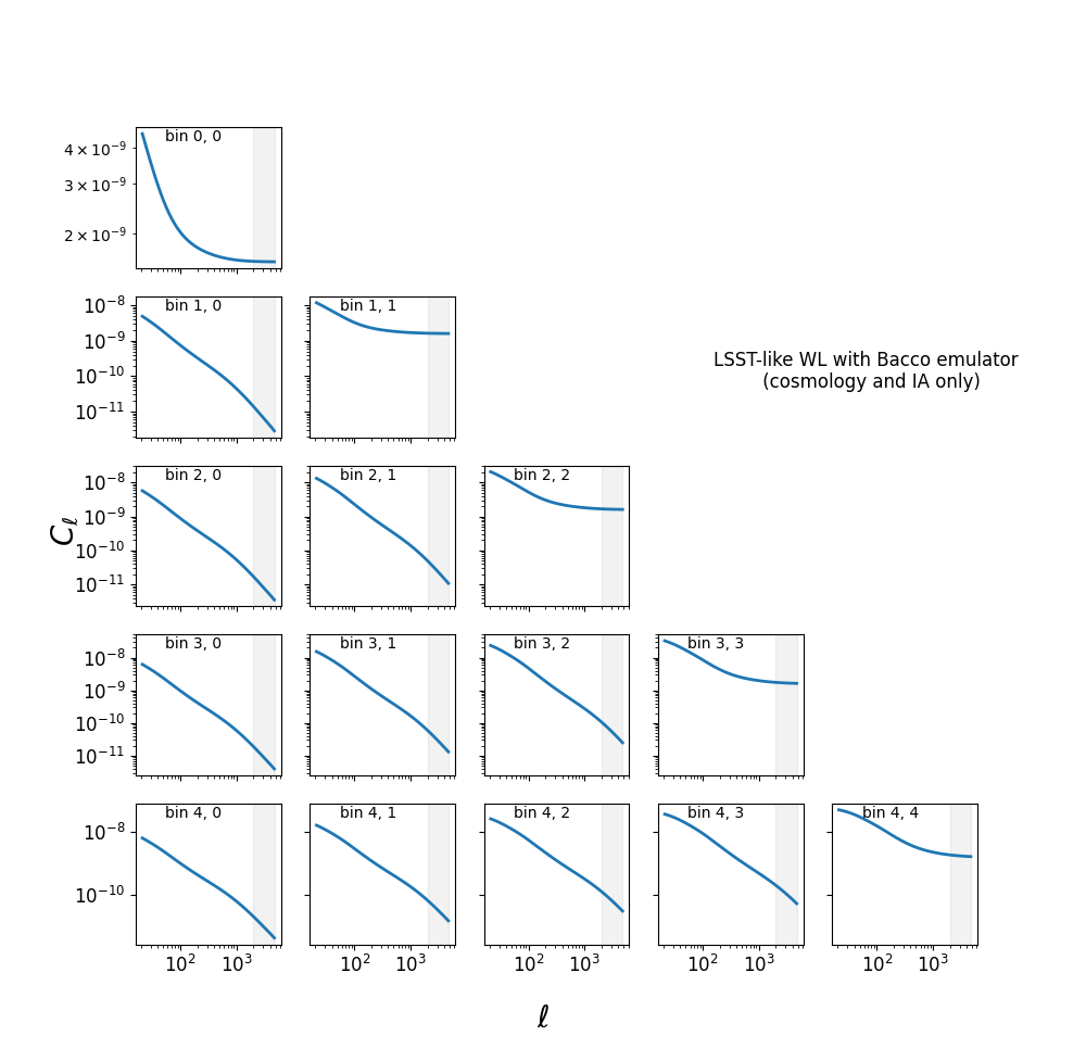
where the grey bands represent the (constant) scale cuts in \(\ell\).

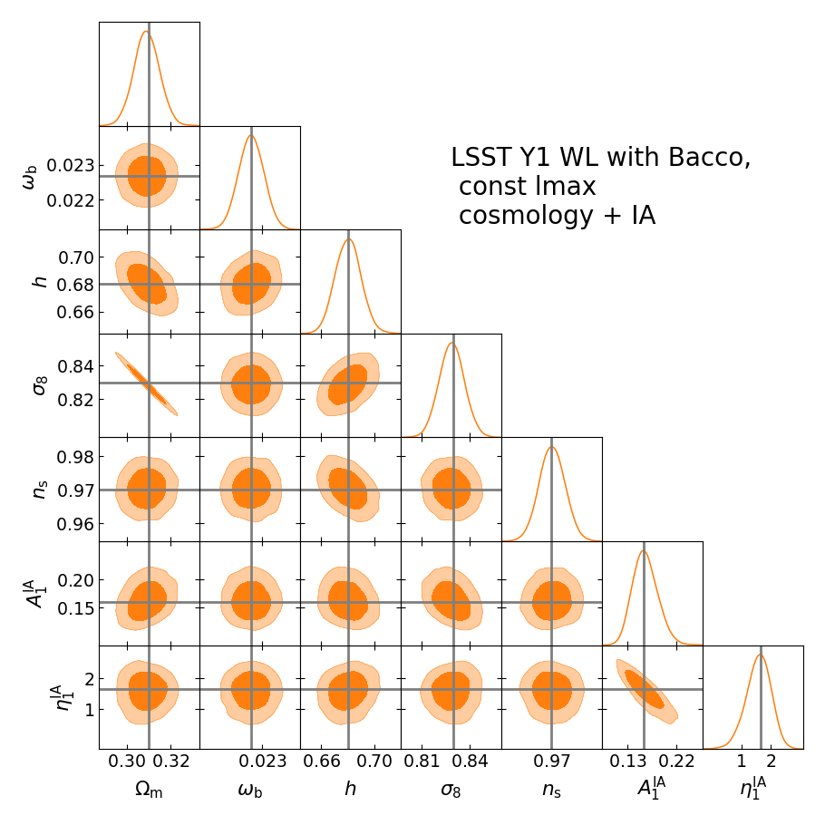
The test code test_mcmc_run.py will instead build a mock catalogue and then run a full MCMC chain analysis with nautilus sampler using parameters, priors and models specified in the input files. The full corner plot with all posterior distributions can be plotted with potting_scripts/plot_posterior.py. The result is a corner plot as the following one: